Introducing aztools

aztools is a collection of tools mostly in python I have been using over the years to analyze telescope X-ray data. I am putting these out so people my find them useful either as a whole as snippets of code. Also, they out here for the sake of the reproducibility of the published work.

The following examples are meant to get you started.

# setup the environment
import numpy as np
import matplotlib.pylab as plt

import aztools as az

# add plot settings
az.misc.set_fancy_plot()

Simulting light curves using the SimLC class

Using the simulation module includes:

• Create a SimLC object, with seed if needed.

• Define the shape of the power spectrum (e.g. powerlaw, broken_powerlaw etc)

• call simulate to generate a random light curve given the defined power spectrum

nlength = 2**16 # number of points desired
dt = 1.0 # sampling time
mu = 10.0 # light curve mean
norm = 'rms' # the normalized of the psd

sim = az.SimLC(seed=393)

# for browen_powerlaw, the parameters are: [norm, index1, index2, break_frequency]
sim.add_model('broken_powerlaw', [1e-5, -1, -2, 1e-3])

sim.simulate(nlength, dt, mu, norm=norm)

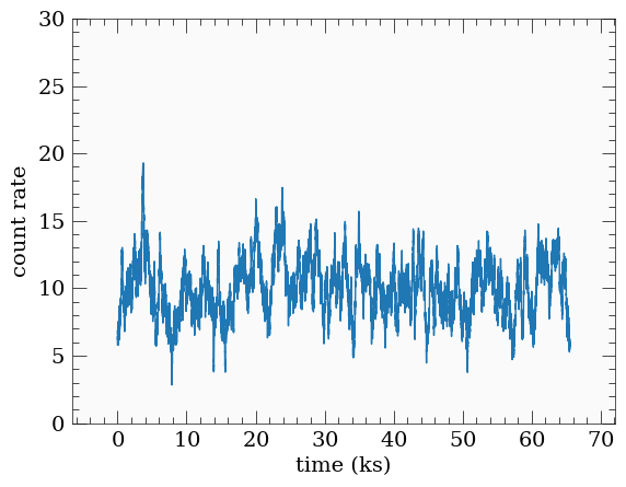
# plot the light curve #
plt.plot(sim.lcurve[0]/1e3, sim.lcurve[1])
plt.xlabel('time (ks)')
plt.ylabel('count rate')
plt.ylim([0, 30])

(0.0, 30.0)

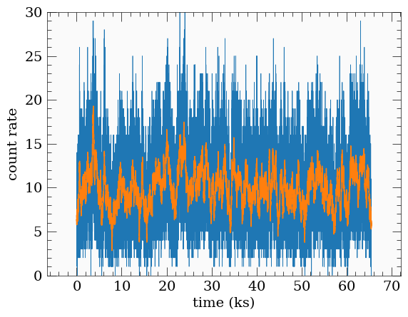
• We can add poisson noise for example

y = sim.add_noise(sim.lcurve[1], deltat=dt, seed=345)
plt.plot(sim.lcurve[0]/1e3, y, lw=0.5)
plt.plot(sim.lcurve[0]/1e3, sim.lcurve[1])
plt.xlabel('time (ks)')
plt.ylabel('count rate')
plt.ylim([0, 30])

(0.0, 30.0)

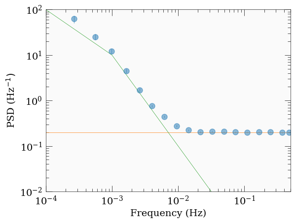
We can now use the LCurve functionality to calculate the power spectrum for example.

First, we calculate the raw psd, then we bin it

The binning is done by az.LCurve.bin_psd, which in turn calls az.misc.group_array of the frequency array, which takes a parameter fqbin that defines the type of binning used. Here, we bin by the number of frequency bin (by_n), starting with 10 frequencies per bin, and increasing it by a factor of 1.5 every time. See az.misc.group_array for details and more grouping options.

az.LCurve.bin_psd returns 4 variables:

• freq: the binned frequency array.

• psd: the binned power spectrum.

• psde: the estimated uncertainty on the binned power spectrum.

• desc: a dict containing some diagnostic useful information about the binning.

# calculate the raw psd #
freq, raw_psd, noise = az.LCurve.calculate_psd(y, dt, norm)

# bin the psd, and we average in log-space #
fqbin = {'by_n': [10, 1.5]}
fq, psd, psde, desc = az.LCurve.bin_psd(freq, raw_psd, fqbin, noise=noise, logavg=True)

# plot the calculated psd.
# also plot the model psd used to generate the light curve in the first place #
plt.errorbar(fq, psd, psde, fmt='o', alpha=0.5)
plt.plot(fq, desc['noise'], lw=0.5)
plt.plot(sim.normalized_psd[0], sim.normalized_psd[1], lw=0.5)
plt.xscale('log')
plt.yscale('log')
plt.xlim([1e-4, 0.5])
plt.ylim([0.01, 1e2])
plt.xlabel('Frequency (Hz)')
plt.ylabel(r'PSD (Hz$^{-1})$')

Text(0, 0.5, 'PSD (Hz$^{-1})$')